Tutorial on DANFIP

Tutorial on DANFIP
Return to Index

Revised 8/18/09

What is it?

Distribution Analysis by Non-linear Fitting of Integrated Probabilities

What's it for?

Analysis of the form of the parent probability distribution of a data set.

What's its advantage?

DANFIP analysis gives a better picture of the form of the parent distribution than does "histogramming"
It extracts the components of multi-component distributions
The reduced Chi-square of the fit can be used to choose between models.
It allows good estimates of population parameters (such as the mean and standard deviation) for truncated distributions

How do you do it?

1) Take a random collection of datum values

2) Sort them in increasing order

3) "Swap" the X and Y axes, so that X = datum value, Y = the rank position in the increasing order of values.

Note: This plot (orange symbols) is called the empirical cummulative distribution function and the Y axis scale represents the number of datum points. This is referred to as the eCDF for short.

If the eCDF is divided by the number of datum points, the Y axis runs from 0 to 1 and it is the shape and scale of the integrated probability function of the parent distribution.

Alternatively, if an integrated probability distribution is multiplied by the number of datum values in a sample, it will be the shape and scale of the eCDF (green symbols).

This FIT between the eCDF and the scaled integrated probability function, IP(y), is what the DANFIP procedure is all about!

For Gaussian (normal) probabilities, this presents a problem since there is no integrated form of the probability distribution function. However, Hasting's approximation formula can approximate the shape of the integrated probability distribution function for any given values of the mean and standard deviation:

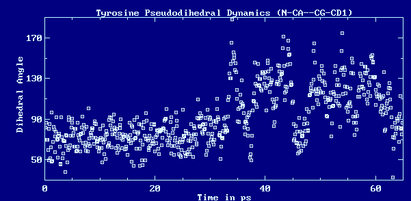
The program DANFIP.EXE (contact author) fits upto six gaussian components to an eCDF using the linear combination of this equation with different means and SD's for each component scaled by their fractional contribution to the whole. For example, consider the following sample from a molecular dynamics simulation:

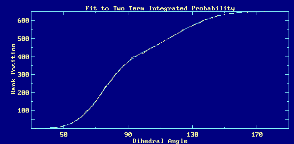
The eCDF of these data fits a distribution function that is the combination of two gaussian subpopulations very well:

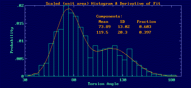
The derivative of the fit curve has the shape of the parent distribution. Scaled to unit area it represents the probability function. The histogram of the data will also have the same shape (also scaled to unit area), but with less definition and more noise.

This information can then be used to interpret the time profile as variations about two mean positions with the "flips" between them occuring sporadically during the course of the trajectory:

One advantage of the DANFIP Approach is that the Chi-square of the fit can be used to select between models:

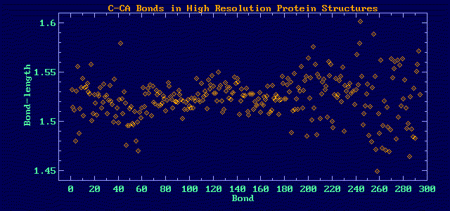
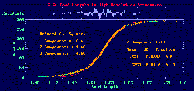
Consider the CA-C (alpha carbon to carboxyl carbon) bond length in high resolution X-ray structures:

This distribution obviously has more than one component. The fits to one, two and three components show that two is sufficient:

In this figure, the data are shown with the orange diamonds, the single gaussian fit is shown in red and the two component fit in green.

When the meter pegs!

Sometimes, measured values are truncated at some lower or higher limit. This occurs often with analog instruments that have fixed readout scales. Sometimes the baseline drifts off scale on the low side or measurements unexpectedly exceed the maximum. Thus, a data set has a number of values recorded either as off scale or assigned to the lowest or highest limiting value.

Truncated data, even if the parent population is gaussian, gives calculated means and standard deviations that are biased.

In this case the sample from the first figure is truncated by assigning any value >270 to have a value of 270. The simulation is from a population with a mean of 250 and a S.D. of 20. The original sample of 200 values gives a mean of 250.4 and S.D. of 19.6. This trucated sample with all data included gives 248.5 and 16.3. If the truncated values are ignored, the values are worse (245.0 and 14.8).

For DANFIP analysis, the values of the data that have been assigned the limiting value are not processed, but the eCDF of the other data is fit WITH THE ORIGINAL SAMPLE SIZE to preserve some of the information. This gives a very good estimate of the parent population parameters (249.7 and 19.4).

For more information about this procedure see Wampler, Analytical Biochemistry 186, 209-219 (1990). Note: Equation 7 in this paper is in Error - by a factor of 2 in the denominator. The correct formula is shown above and the presentation linked below.

For the slides of a siminar presentation concerning this process, follow this link.

An implementation of the full DANFIP procedure in Quick Basic 64 (http://www.qb64.net/) that runs on Window versions up through 8 is available from the author. The Levenberg-Marquardt fitter in this implementation is streamlined for quicker execution (however, the algorithm used does make it a bit less likely to converge if the initial guesses are not too good).

Return to Home Page